Solve the following problem:
Referring to Example 1:
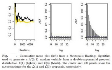
a. Write a Metropolis-Hastings algorithm to produce Figure . Note that n L(a) random variables can be generated at once with the R command
> ifelse(runif(n)>0.5, 1, -1) * rexp(n)/a
b. What is the acceptance rate for the Metropolis-Hastings algorithm with candidate L(3)? Plot the curve of the acceptance rates for L(α) candidates when α varies between 1 and 10. Comment.
c. Plot the curve of the acceptance rates for candidates L(0, ω) when ω varies between .01 and 10. Compare it with those of the L(α) candidates.
d. Plot the curve of the acceptance rates when the proposal is based on a random walk, Y = X(t) + ε, where ε ∼ L(α). Once again, compare it with the earlier proposals.
Example 1:
In an Accept-Reject algorithm generating a N (0, 1) sample from a double-exponential distribution L(α) with density g(x|α)=(α/2) exp(-α|x|), the choice α = 1 optimizes the acceptance rate . We can use this distribution as an independent candidate q in a Metropolis-Hastings algorithm. Figure compares the behavior of this L(1) candidate along with an L(3) distribution, which, for this simulation, produces an inferior outcome in the sense that it has larger autocovariances and, as a result of this, slower convergence. Obviously, a deeper analysis would be necessary to validate this statement, but our point here is that the acceptance rate (estimated) for α = 1 is twice as large, 0.83, as the acceptance rate (estimated) for α = 3, 0.47.
