The Fourier transform is a powerful tool for converting time-series data into its frequency components for the purpose of signal analysis and processing.
Background
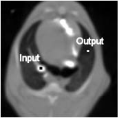
In this assignment, you are given a file called "PBF.txt" which is actual pulmonary blood flow data acquired by computed tomography (CT) imaging of porcine animal models. The data was obtained by a 1-second bolus injection of non-iodinated contrast agent into the right ventricle (RV). Due to mixing in the RV, the bolus is "low-pass filtered" and results in a unimodal input function, x(t), measured in the pulmonary artery (PA) using CT imaging.

This input function traverses from the PA through various arterial pathways and eventually reaches the lung parenchyma (i.e. microvascular beds within the lung). The extent to which contrast flows to the microvascular beds can also be measured using CT techniques.
Assignment
Download the "PBF.txt" file. In the file, you will find four columns:
(1) time data (unit: seconds),
(2) input function, x(t), measured at the pulmonary artery (unit: Hounsfield Unit (HU)),
(3) output function, y(t), measured in the lung parenchyma (unit: Hounsfield Unit (HU)),
(4) transfer function, h(t), which describes the system which modifies the input from the PA and produces the output seen at the lung parenchyma.
Using Matlab:
- Plot x(t), y(t), and h(t), each vs. time.
- In the time domain, descriptively analyze the how the x(t) differs from y(t).
- Perform a Fourier Transform (Matlab command, fft(x)) of x(t), and y(t). Plot the magnitude (i.e. "abs") of the FFTs of the input (x(t)) and output (y(t)). (Note: Using the FFT function, you will obtain an output that has both real and imaginary components).
- Determine how many frequencies are needed to adequately (respectively within +1% and +5% error) represent the original time series data (analyze for both x(t) and y(t)).
Hint: (1) You will need to use the IFFT function to perform the "inverse FFT" to go from the frequency domain back to the time domain)
(2) Error= sum(abs(x(t))-abs(x_new(t)))/sum(abs(x(t))) x and x_new are the original time history and new one generated by IFFT
- Plot the original vs. the "truncated" waveforms that you generate for each.
- Comment/discuss your observations.
- Using the transfer function, h(t), convolve your new input function with the transfer function and compare the output with the original output (y(t)) and your new output function. (Hint: Use the CONV command in Matlab. Using CONV, the length of the new data will be twice as long as the original vector. Only plot the first half).
Download:- PBF.txt