Solving the dynamics of the pendulum

Question

Problem Statement
Assume that a simple pendulum is attached to our spring-damper-mass system. A simple schematic of the model is given in Figure .

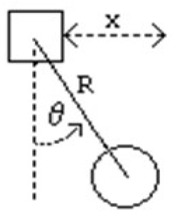
The mass can move horizontally where as the pendulum oscillates about a vertical axis attached to this mass.

The problem parameters in their appropriate units are given below in Table.

     Variable              Description            Value
       M               Mass of the body         1.0
       m          Mass of the pendulum       1.0
       k             Spring constant              10.0
      c             Damping Coefficient          0.5
      R         Length of the pendulum        1.0

The equation of motion of the system can be written as:
(M+msin² θ)x'' cx'+kX-mR(θ')² sinθ-mgsinθcosθ=0

(M+msin² θ)R θ''-cx'cos θ-kxcos θ+mR(θ')²sinθcos θ + (m+M)gsin θ=0

with initial condition x(0)=0 x'(0)=0 θ(0)=10°   θ'(0)=0

1. By defining new variables rewrite the equations of motion in the form y '= f (t , y )
2. Solve for the dynamics of the resulting system for 20 seconds of real time using midpoint method. Choose your step size so that the local error is less than 10^-4.

3. Plot x vs. t, θ vs. t and θ vs. x on three separate figures.
4. Repeat steps 2 and 3 for θ(0)=90^o and  θ(0)=179^o while keeping the other initial conditions fixed.

Note: Don’t forget to convert the angles to radians.

Assignment
1. Develop a Matlab function named RK4.m which implements the classical 4-stage Runge-Kutta method (RK-4) for solution of IVPs.
2. Do again steps 2 and 3 by using the RK-4 method as the solution technique. Compare the step sizes used and the CPU times spent by the Mid-point and RK-4 methods.