Response to the following :
Referring to Example 1:
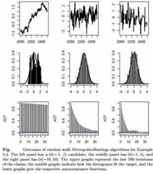
a. Reproduce the graphs in Figure for difference values of δ. Explore both small and large δ's. Can you find an optimal choice in terms of autocovariance?
b. The random walk candidate can be based on other distributions. Consider generating a N (0, 1) distribution using a random walk with a (i) Cauchy candidate, and a (ii) Laplace candidate. Construct these Metropolis-Hastings algorithms and compare them with each other and with the Metropolis-Hastings random walk with a uniform candidate.
c. For each of these three random walk candidates, examine whether or not the acceptance rate can be brought close to 0.25 for the proper choice of parameters.

Example 1:
The historical example of Hastings (1970) considers the formal problem of generating the normal distribution N (0, 1) based on a random walk proposal equal to the uniform distribution on [-δ, δ]. The probability of acceptance is then

Figure describes three samples of 5000 points produced by this method for δ = 0.1, 1, and 10 and clearly shows the difference in the produced chains: Too narrow or too wide a candidate (that is, a smaller or a larger value of δ) results in higher autocovariance and slower convergence.
Note the distinct patterns for δ = 0.1 and δ = 10 in the upper graphs: In the former case, the Markov chain moves at each iteration but very slowly, while in the latter it remains constant over long periods of time.