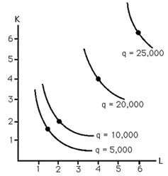
1) The above figure shows the isoquants for producing steel. Increasing returns to scale are
A) present when producing less than 10,000 tons.
B) present when producing less than 20,000 tons.
C) present when producing less than 30,000 tons.
D) never present.
2) The above figure shows the isoquants for producing steel. Decreasing returns to scale are
A) present when producing more than 10,000 tons.
B) present when producing more than 20,000 tons.
C) present when producing more than 30,000 tons.
D) never present.
3) The above figure shows the isoquants for producing steel. Constant returns to scale are
A) present when producing less than 10,000 tons.
B) present when producing between 10,000 and 20,000 tons.
C) present when producing more than 20,000 tons.
D) never present.
4) The above figure shows the isoquants for producing steel. When producing more than 20,000 tons there are
A) increasing returns to scale.
B) decreasing returns to scale.
C) constant returns to scale.
D) economies of scale.
5) The above figure shows the isoquants for producing steel. When producing less than 10,000 tons there are
A) increasing returns to scale.
B) decreasing returns to scale.
C) constant returns to scale.
D) diseconomies of scale.
6) The above figure shows the isoquants for producing steel. When producing between 10,000 and 20,000 tons there are
A) increasing returns to scale.
B) decreasing returns to scale.
C) constant returns to scale.
D) economies of scale.

7) The above figure shows the isoquants for the production of steel. In which regions of production are there increasing, decreasing, and constant returns to scale?
8) Short-Run Production: One Variable and One Fixed Input

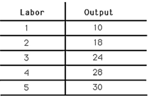
1) The above figure depicts a short-run production function for Albert's Pretzels. The marginal productivity of labor
A) rises then falls as the amount of capital increases.
B) falls then rises as the amount of labor increases.
C) is greater than or equal to the average productivity of labor for all amounts of labor.
D) is less than or equal to the average productivity of labor for all amounts of labor.
2) The above figure shows the short-run production function for Albert's Pretzels. The marginal productivity of labor for the third worker is
A) 6.
B) 8.
C) 24.
D) not known from the information provided.
3) The above figure shows the short-run production function for Albert's Pretzels. The marginal productivity of labor equals the average productivity of labor
A) for all levels of labor.
B) at none of the levels of labor.
C) only for the first worker.
D) only for the fifth worker.
4) The above figure shows the short-run production function for Albert's Pretzels. The law of diminishing marginal productivity
A) appears with the second worker.
B) has not yet appeared for any of the levels of labor.
C) first appears with the fifth worker.
D) is refuted by this evidence.
5) The above figure shows the short-run production function for Albert's Pretzels. The average product of labor
A) increases first and then decreases.
B) decreases first and then increases.
C) decreases throughout.
D) increases throughout.
9) Explain why the marginal cost curve intersects a U-shaped average cost curve at its minimum point.
10) Suppose the total cost of producing T-shirts can be represented as TC = 50 + 2q. The marginal cost of the 5th T-shirt is
A) 2.
B) 10.
C) 12.
D) 60.
11) Suppose the total cost of producing T-shirts can be represented as TC = 50 + 2q. The average cost of the 5th T-shirt is
A) 2.
B) 12.
C) 52.
D) 60.
12) Suppose the total cost of producing T-shirts can be represented as TC = 50 + 2q. Which of the following statements is TRUE at all levels of production?
A) MC = AVC
B) MC = AC
C) MC > AFC
D) All of the above.
13) Suppose the short-run production function is q = 10 * L. If the wage rate is $10 per unit of labor, then AVC equals
A) q.
B) q/10.
C) 10/q.
D) 1.
14) Suppose the market for grass seed can be expressed as
Demand: QD= 100 - 2p
Supply: QS = 3p
At the market equilibrium, calculate the price elasticities of supply and demand. Use these numbers to predict the change in price resulting from a specific tax.
15) The principle that "More is better" results in indifference curves
A) sloping down.
B) not intersecting.
C) reflecting greater preferences the further they are from the origin.
D) All of the above.
16) There is an indifference curve through every bundle because of the assumption of
A) transitivity.
B) completeness.
C) rationality.
D) nonsatiation.
17) Indifference curves are downward sloping because of the assumption of
A) completeness.
B) transitivity.
C) more is better.
D) All of the above.
18) If two indifference curves were to intersect at a point, this would violate the assumption of
A) transitivity.
B) completeness.
C) Both A and B above.
D) None of the above.
19) Indifference curves that are thick violate
A) the assumption of transitivity.
B) the assumption that more is better.
C) the assumption of completeness.
D) none of the assumptions.
20) A consumer's willingness to trade one good for another can be expressed by the consumer's
A) indifference curve.
B) marginal rate of substitution.
C) Both A and B above.
D) None of the above.
21) Convexity of indifference curves implies that consumers are willing to
A) give up more "y" to get an extra "x" the more "x" they have.
B) give up more "y" to get an extra "x" the less "x" they have.
C) settle for less of both "x" and "y".
D) acquire more "x" only if they do not have to give up any "y".
22) Measuring "y" on the vertical axis and "x" on the horizontal axis, convexity of indifference curves implies that the MRS of "y" for "x"
A) is decreasing as "x" increases.
B) is increasing as "x" increases.
C) is constant as "x" increases.
D) cannot be calculated for large levels of "x".
23) Suppose the short-run production function is q = 10 * L. If the wage rate is $10 per unit of labor, then MC equals
A) q.
B) q/10.
C) 10/q.
D) 1.
24) If average cost is decreasing
A) marginal cost equals average cost.
B) marginal cost exceeds average cost.
C) marginal cost is less than average cost.
D) Not enough information
25) If average cost is positive
A) marginal cost equals average cost.
B) marginal cost exceeds average cost.
C) marginal cost is less average cost.
D) Not enough information is given.
26) Suppose the short-run production function is q = L0.5. If the marginal cost of producing the tenth unit is $5, what is the wage per unit of labor?
A) $1
B) $0.5
C) $0.25
D) It cannot be determined without more information.
27) Suppose the short-run production function is q = 10 * L. If the wage rate is $10 per unit of labor, then AFC equals
A) 0.
B) 1.
C) 10/q.
D) It cannot be determined from the information provided.
28) When a firm produces one unit, the variable cost is $3. When the firm produces two units, the variable cost is $6. What is the marginal cost associated with two units of production?
A) $2
B) $0.5
C) $6
D) $3