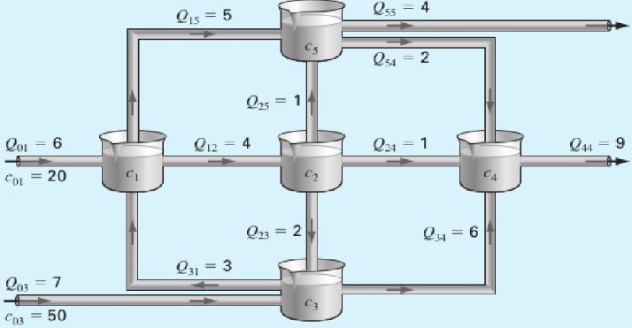
1. Five reactors linked by pipes are shown in the following figure. The rate of mass flow through each pipe is computed as the product of flow (Q) and concentration (c). At steady state, the mass flow into and out of each reactor must be equal. For example, for the first reactor, a mass balance equation can be written as Q01c01 + Q31c3 = Q15c1 + Q12c1.

a) Write mass balance equations for the remaining 4 reactors. Put the known values in the 5 equations and convert each equation into a form where left hand side contains all the variables and the right hand side the constant term.
b) Express the equations in the matrix form Ax = b. Show each of the three matrices i.e the coefficient matrix, the variable matrix and the constant matrix.
c) Perform LU factorisation of A using MATLAB. Show commands that you run and the lower triangular matrix L, the upper triangular matrix U and the permutation matrix P.
d) Then use L,U,P matrices in MATLAB to find the values of the variables in your equations. Show your commands and their output.
e) If c03 = 60 and c01 = 30, perform the minimum tasks on MATLAB to find the values of the variables. Show your commands and their output.
2. In numerical integration and in many other cases, we need a polynomial named Legendre polynomial. Often the zeros i.e. the roots of the polynomial are also needed. The sixth order Legendre polynomial is given by the following equation:
P6(x) = 693x6 – 945x4 + 315x2 – 15
There are six roots of the P6(x) = 0 equation. Note that all the zeros of Legendre polynomial have magnitude less than one i.e. the roots are between -1 and 1. Also, note that for a polynomial of even order, the zeros are symmetrical about the origin. Therefore, for each root x, -x is also a root. If you find the three roots between 0 and 1, the other roots are negative of them.
Now write a MATLAB program that does the following:
a) Plot the given function in MATLAB for x ranging from -1 to 1. Put a proper title of the plot, also label the axes appropriately.
b) Use MATLAB's roots function to obtain the six roots of the equation. Display the roots and plot them with different colors and symbols on the same chart where you plotted the function.
c) Write a MATLAB program segment that will implement the root finding algorithm by Newton-Raphson method. Newton-Raphson method needs one initial value to run each time. You program segment will be executed with different initial values that you get from d).
d) Use a loop in your program to execute the Newton-Raphson program segment for each initial value between -1 to 1 with an interval 0.1. Plot the initial values on the x-axis with the color that you used in b) to plot the root obtained from this initial value; these plots will be on the same chart. For example, if you start from 0.1 and obtain the first root that you plotted by using color red in b), then plot (0.1, 0) with color red.
e) In the plot, you will see one root is obtained from an initial value that is close to another root. Can you explain by observing the plot why that is happening.
3. Consider the following three sets of equations.
8x + 3y + z = 12
-6x + 7z = 1
2x + 4y -z = 5
x + y + 5z = 7
x + 4y -z = 4
3x + y – z = 3
-x + 3y + 5z = 7
-2x + 4y -5z = -3
2y -z = 1
a) Write all of the above sets of equations in the matrix format and identify the sets that you cannot solve by using an iterative method such as Jacobi and/or Gauss-Seidel method. Show the details of how you decide that the method will not converge for the identified set.
b) If there is any set in the above three that will converge, select that (or any one if more than one exists) and manually show as many steps as you need for the Jacobi Method to achieve an absolute approximate relative error level for each variable below 5%.
c) Using the same set of equations that you used in b), manually show as many steps as you need for the Gauss-Seidel method to obtain the absolute approximate relative error level for each variable below 5%. While following Gauss-Seidel method steps, describe where you are doing different from that you did in case of the Jacobi method.
d) Consider the number of steps required in Jacobi Method and in Gauss-Seidel method to achieve the same quality (in terms of absolute approximate relative error to be below 5%) solutions. Which method is more efficient in the number of steps? Can you explain why that method is more efficient than the other?
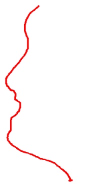
4. The figure below is an example profile of a man. Instead of the profile, you can also use a unique (different to every one else's) profile (e.g. car, boat) of your own from any other source.

a) Include the original photograph of your selected profile with your assignment. Trace your drawing on a graph paper. For convenience you can rotate the given profile.
b) Locate 20 points on the profile. You should select more points where the profile is more curvy, and few points where the profile is almost linear. Display these points in MATLAB output and on MATLAB chart with color blue but no lines to join them.
c) You will use MATLAB polyfit and polyval functions to find one polynomial with all points. Now plot the profile with your fitted polynomial; you should plot more points on the polynomial in this case. Use a different color.
d) Try different numbers of points from your tracing for polyfit and different numbers of points for polyval to plot them. Show at least five different attempts. You will plot these 5 attempts using 5 different colors. Make these attempts in such as way that the best plot looks as much alike as possible to the original profile given.
5. A circular shaft has a diameter, d (m), that varies with axial position, x (m), along the shaft (from the support position at x = 0 m). The variation is given by d = 0.02e-x(1+x2) where 0 ≤ x ≤ 3 m. An axial load P = 40kN is applied to the end of the shaft, whose Modulus Elasticity E = 2*1011Nm-2. The axial elongation of the ΔL (m) of the shaft in the range of values of 0 ≤ x ≤ 3 m is given by: ΔL = P/E ∫4dx/(πd2).

a) Using MATALB, plot the shaft diameter with axial position. Use appropriate labels.
b) Use MATLAB integration techniques to determine the total Axial Elongation.
c) Explain the theory of Simpson 1/3 rule for integration in detail. Use appropriate examples to demonstrate how it works and how the integration result is computed.
The effective average DC equivalent value of an alternating current is given by the formula:
IRMS = √(T-1∫[i(t)]2dt)
where i(t) is the instantaneous current (A) and T is the waveform period (s) and the lower and the upper limits of the integration are 0 and T. The current within a circuit (which replicates every 5 ms) is given by:
i(t) = 10e-t/5sin(2πt/5) (mA)
a) Using MATALB, plot the circuit current i(t) over four periods. Use appropriate labels.
b) Use MATLAB integration techniques to determine the equivalent DC current (RMS) within the circuit.
c) Describe the theory of Simpson 1/3 rule for integration in detail. Use suitable examples to demonstrate how it works and how the integration result is computed.