Question 1
Introduction
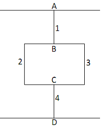
You are designing a pipe network system that transfers water from the upper pipe to the lower pipe. Note that Figure 1 is a plan view and the elevation is constant across all pipes. The static pressure difference between points A and D is designed to be PA - PD = 3 atm (1 atm = 1 standard atmospheric pressure = 101.3 kPa). It is necessary to ensure that the speed of the flow through every pipe is at least 2 m/s so that there is no sediment build-up. Determine if this is the case.
Theory
The change in pressure between two points along a streamline (a flow path) is modelled by the Bernoulli equation

where P is the static pressure, Ρ the density, V the speed, g gravitational acceleration, h the elevation and ΔΡloss is the reduction in pressure due to any losses in the system. The most important loss (and the only one to be accounted for here) is caused by friction:
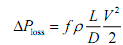
where f is the Darcy-Weisbach friction factor. Fluid flow is governed by the continuity equation (which is conservation of mass); for incompressible (constant-density) flow, this is:
Q = VA = Const
where Q is the volume flow rate (m3/s) and A is the cross-sectional area. Incompressible flow is a good assumption for liquids. A consequence of Eq. (3) for Eq. (1) is that if the cross-sectional area is constant for a given pipe, the flow speed at the start is equal to the speed at the end and can be defined based on the pipe ID rather than an end-point ID.
Pipe networks can be considered to be equivalent to electrical circuits in series and parallel, with pressure change equivalent to potential difference and volume flow rate equivalent to current.
However, the resistance cannot be treated as constant: it is a non-linear function of the flow speed. The rules of potential difference and current are still maintained however:
a) The pressure change (potential difference) across multiple branches in parallel is equal (e.g. PB - PC is the same regardless of whether pipe 2 or 3 is taken).
b) The sum of the volume flow rates (currents) entering a junction is equal to the sum of the volume flow rates exiting a junction (e.g. Q1 = Q2 + Q3).
Because of the non-linear nature of the system [flow rate is squared in Eq. (1) and f is a non-linear function of Q], iteration is required to determine the flow speeds in each pipe section. To do this, certain constraints can be applied based on the rules of potential difference and current:
1. The pressure change between points A and D is known and is equal to the sum of the pressure changes along all pipes in series that connect points A and D. This constraint should be used only once.
2. The pressure change across pipes in parallel is the same for each pipe.
3. The sum of volume flow rates entering junction B is equal to the sum of volume flow rates exiting B; similarly for C.
These constraints provide a set of equations that can be solved for the speeds in each pipe.
To calculate the friction factor, the common formula that is used is the Colebrook formula (Colebrook 1938-39):
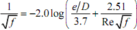
where e is the absolute roughness of the pipe wall and the Reynolds number is
with v (the Greek letter "nu") the kinematic viscosity. Equation (4) is only valid for turbulent pipe flow (Re > 2300), otherwise f = 64/Re. The Moody diagram (Figure 2) is a standard method of determining f (the left axis) for hand calculations; the range of possible values for f given the different blue lines that represent the range of plausible pipe roughnesses can be seen.
Requirements
For this assessment item, you must produce MATLAB code which:
1. Iterates until convergence is reached (the previous guess for the velocities is not significantly different from the current guess).
2. Calculates the friction factor for the current guess of velocities.
3. Reports the flow velocity in each pipe to the Command Window in addition to confirming that the speeds meet the required level
4. Validates the code by checking that the volume flow rates in the branches are consistent.
5. Verifies the code by ensuring that the friction factor calculation is valid.
6. Displays to the Command Window a brief discussion (fewer than 5 lines) stating the value you selected for the under-relaxation factor and why you selected that value.
7. Has appropriate comments throughout.
An important component of quality assurance is to test (verify) that each function works correctly:
8. Write a test program that supplies block of code with a known input and confirm (verify) that the output is correct. (Writing blocks of code as functions makes the code more transparent, more portable and easier to test!)
Attachment:- matlab.rar