General methodology used by econometricians

Question

Question: Following the general methodology used by econometricians as explained in the session for week 1 (eight steps), explain how you would proceed to determine if a good complies with the Law of Demand.

Question: Find out how the Ordinary Least Squares (OLS) method estimates b1 and b2 for the simple linear equation (Y = B₁ + B₂ X). Once you had estimated the equation, elucidate how you would determine whether it is a good fit for the actual equation.

Question: Analyzing data at country level, Helble and Sato (2011) estimated the given relationship between the alcohol consumption per capita (Alc) and the growth rate of GDP per capita (gGDP).

Alc = 4.198 + 0.088 gGDP                    
R² = 0.004,
n = 4829
Standard error = (0.144) (0.031)

a) Set up a 95% confidence interval for the slope (B₂).
b) Using the confidence interval computed in (a) test the hypothesis that B₂=0.
c) Test the significance at 5% of B₂ by means of the t-test.  
d)  Discuss the relationship this equation reflects, elaborating on the meaning of the R², and the result of the t-test.

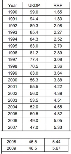
Question: In the table below you can find data on the recommended retail price for a 20 cigarette pack (RRP, pounds sterling) and UK consumption of cigarettes (UKDP, in billion cigarettes) for 20 years. Data is sourced from the Tobacco Manufacturers' Association.

a) Discuss the relationship, if any, you would expect between the two variables.
b) Draw the scatter plot between UKDP and RRP.
c) Do an OLS regression, interpret and discuss your results fully. 
d) Establish a 95% confidence interval for the slope and test the hypothesis that the true slope coefficient is zero.
e) Suppose the government decides to increase tax so that the RRP reaches £6. Forecast consumption at this price level.

Question:

a) Design a simple econometric project to identify the factors that affect the demand for a good or service of your preference. Estimate the significance of these factors using multiple regression analysis (at least two explanatory variables) and using at least 20 data points. Use a full range of econometric techniques in your project including estimating your model using absolute values and natural logs of these values.

Interpret the coefficients, their individual statistical significance, joint significance, and model goodness-of-fit in order to evaluate the usefulness of the econometric techniques in identifying the factors that affect demand.

b) Estimate the demand equation in (a) with only one explanatory variable and compare your results with those in (a) identifying the consequences of this type of specification error.

Question:

a) Give two examples of economic variables that can introduce a multi-collinearity problem into your OLS estimation and two other examples for heteroscedasticity.

b) Discuss the problems and practical issues both multicollinearity and heteroscedasticity may create on the variables you have chosen in (a).

c) Briefly explain the possible solutions you could apply to resolve the issues identified in (b).

Question: The following equation is estimated to assess the effects of gender and education on wages (standard errors in brackets):

ln(wage) = 0.389 – 0.227 female + 0.082 educ – 0.0056 female . educ
(0.119)  (0.168)             (0.008)          (0.0131)
n = 526, R² = 0.441

Where wage is the wage in dollars per hour, female is a dummy variable indicating female gender (1) or otherwise (0), and educ is the years of education.

a) Interpret the equation and the goodness-of-fit.
b) Test the individual significance of the coefficients for female, educ, and the interaction effects at the 1%, 5%, and 10% levels.
c) Is this estimation likely to be affected by autocorrelation? Explain why.