Discuss the below:
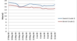
Q1) Use the per-barrel oil price data provided above to create a line chart using Excel that plots both prices. Be sure that the date is on the X-axis and the price in dollars is on the Y-Axis.
|
Date
|
Sweet Crude $
|
Brent Crude $
|
|
17-May-90
|
18.89
|
17.05
|
|
18-May-90
|
18.78
|
17.08
|
|
21-May-90
|
18.26
|
16.65
|
|
22-May-90
|
17.51
|
16.48
|
|
23-May-90
|
16.25
|
15.7
|
|
24-May-90
|
16.02
|
15.8
|
|
25-May-90
|
16.12
|
15.95
|
|
29-May-90
|
18
|
15.48
|
|
30-May-90
|
17.88
|
15.98
|
|
31-May-90
|
17.47
|
15.3
|
|
1-Jun-90
|
17.51
|
15.43
|
|
4-Jun-90
|
17.09
|
15.35
|
|
5-Jun-90
|
16.41
|
14.78
|
|
6-Jun-90
|
16.91
|
14.8
|
|
7-Jun-90
|
16.65
|
15.03
|
|
8-Jun-90
|
16.78
|
14.68
|
|
11-Jun-90
|
16.82
|
14.73
|
|
12-Jun-90
|
17.39
|
14.95
|
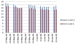
Q2) Use the per-barrel oil price data provided above to create a Bar chart using Excel that plots both prices. Be sure that the date is on the X-axis and the price in dollars is on the Y-Axis.

Q3) Create descriptive statistics including mean, mode, median, range, high, low, variance and standard deviation for the two different oil prices above. Comment on the similarities and differences.
Sweet Crude

|
Date
|
Sweet Crude
|
Descriptive Statistics for Sweet Crude
Mean:
17.26
Median:
17.24
Mode:
17.51
Range:
2.87
Standard Deviation:
.8617
Sample Variance:
.7425
|
Date
|
Brent Crude
|
Descriptive Statistics for Brent Crude
Mean:
15.62
Median:
14.96
Mode:
0
Range:
2.40
Standard Deviation:
1.036
Sample Variance:
1.074
|
|
24-May-90
|
16.02
|
8-Jun-90
|
14.68
|
|
25-May-90
|
16.12
|
11-Jun-90
|
14.73
|
|
23-May-90
|
16.25
|
5-Jun-90
|
14.78
|
|
5-Jun-90
|
16.41
|
6-Jun-90
|
14.80
|
|
7-Jun-90
|
16.65
|
12-Jun-90
|
14.95
|
|
8-Jun-90
|
16.78
|
7-Jun-90
|
15.03
|
|
11-Jun-90
|
16.82
|
31-May-90
|
15.30
|
|
6-Jun-90
|
16.91
|
4-Jun-90
|
15.35
|
|
4-Jun-90
|
17.09
|
1-Jun-90
|
15.43
|
|
12-Jun-90
|
17.39
|
29-May-90
|
15.48
|
|
31-May-90
|
17.47
|
23-May-90
|
15.70
|
|
1-Jun-90
|
17.51
|
24-May-90
|
15.80
|
|
22-May-90
|
17.51
|
25-May-90
|
15.95
|
|
30-May-90
|
17.88
|
30-May-90
|
15.98
|
|
29-May-90
|
18
|
22-May-90
|
16.48
|
|
21-May-90
|
18.26
|
21-May-90
|
16.65
|
|
18-May-90
|
18.78
|
17-May-90
|
17.05
|
|
17-May-90
|
18.89
|
18-May-90
|
17.08
|
Q4) What is the kurtosis (research kurtosis on your own) and skew of the two oil prices shown above? What does this mean? Explain
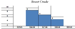
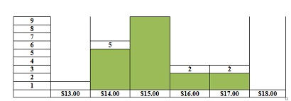
Q5) Create a histogram for each of the two oil prices shown.
Sweet Crude


Q6) Does the data seem closer to being normal (empirical rule) or not? Use your answers from problems 1-5 above to explain
Q7) Your employer, Woodbridge Electric Inc., wants to offer a warranty on the new compact fluorescent light bulb that they have produced and tested. You are called into a meeting and operational experts provide the following data: mean bulb life = 8000 hours, standard deviation = 400 hours (assume a normal distribution). The financial people tell you that the firm cannot afford to replace more than 2.5% of the bulbs under warranty. Some members of the board of directors are pressuring you to come up with a warranty of 7000 hours. The marketing people are pressuring you to create a warranty of 7500 hours. Use the data and adhere to the 2.5% financial constraint above to make your calculations and recommend the highest warranty that you can. What do you recommend as a warranty?
Q8) Why did you choose this figure as the warranty? What percentage of bulbs would need to be replaced if you chose a warranty of 7000 or 7500? Justify your answer statistically. How do you explain this to the board of directors, marketing people and financial people?
Q9 )The Operational experts of Woodbridge Electric have announced a breakthrough in the production process and the mean of the same bulb has increased to 9000 hours and the standard deviation has decreasing to 200 hours (again assume a normal distribution). Using the same 2.5% constraint how does this affect the warranty? Is this good news or bad for the customers and the firm?