A pressure composition diagram for a liquid vapor system can be used to show the composition of the liquid and equilibrium vapor.
Vapor equilibrium data are useful in the study of distillations. It is of value to have diagrams showing not only the vapor pressure of a solution of given composition but also the composition of the vapor that is in equilibrium with the liquid. This additional information can be put on the vapor-pressure composition diagrams.
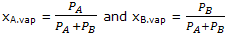
Since the partial pressures of gas components are proportional to the number of moles of gases per unit volume, the mole fractions of the vapor can be written
for an ideal solution Raoult's law is obeyed and
PA = xAP°A and PB = xBP°B
Thus for an ideal solution the vapor composition is given by

this expression can be used to calculate the compositions of vapor in equilibrium with an ideal solution of any composition. The qualitative result is that the vapor will be relatively richer in A ifP°A is greater than P°B, that is, if A is the more volatile component.
The vapor-composition information is added to the vapor pressure composition diagram by allowing the abscissa to be used for both liquid and vapor compositions, as illustrated for ideal solution. at a particular vapor pressure one can read, along the horizontal dashed line, for example, the composition of the liquid that gives rise to this vapor pressure and also the composition of the vapor that exists in equilibrium with this liquid. More often one uses the diagram by starting with a given liquid composition, a reading off the vapor pressure of this solution and obtaining the composition b of the vapor in equilibrium with the solution.
For nonideal solutions, the composition of the vapor in equilibrium with a given solution must be calculated from equation and the experimentally determined vapor pressures of the two components. The vapor pressures of the two components of representative nonideal solutions were shown. The vapor compositions over an acetone chloroform solution containing a chloroform mole fraction of 0.2 can be calculated as an example. At this concentration, the vapor pressure of chloroform is, 0.046 bar, and that of acetone is 0.355 bar. The total vapor pressure is 0.401 bars. The mole fraction of chloroform in the vapor is 0.046/0.401 = 0.115; that of acetone is0.885. such data can be used to add the vapor composition curves.
It is helpful to notice and remember that on vapor pressure composition diagrams (both for ideal and any type of nonideal system) the liquid composition curve always lies above the vapor composition curve. Where the curve for the vapor pressure of the liquid shows a maximum or minimum, however the equilibrium vapor has the same composition as the liquid. Such points will be important when a separation process is considered.
The diagrams show the phase or phases present at any pressure at the specified temperature. Consider, for example, a point in the lower region of any of these figures. The pressure is lower than the vapor-pressure curves, and the system exists as a vapor. As the pressure is increased, the point describing the system moves up until it reaches the vapor-composition line. The vapor is then in equilibrium with liquid of the composition given by the liquid composition curve at that pressure. Attempts to increase the pressure will produce more liquid. In general, the liquid composition will be different from that of the vapor. When this process is complete the system is represented by a point on the upper liquid composition curve. Further pressure increases merely increase the pressure on the liquid. It follows from this discussion that the three regions can be labeled "vapor", "vapor and liquid", and "liquid".